Weights and Activation Quantization (W4A16)

Learning Objectives

By completing this exercise, you will:

Understand W4A16 quantization and its benefits for LLM optimization
Learn to set up a complete quantization pipeline using OpenShift AI
Gain hands-on experience with SmoothQuant and GPTQ quantization techniques
Evaluate quantized model performance and memory efficiency

Overview

In this exercise, you will use a Jupyter notebook to investigate how LLM weights and activations can be quantized to W4A16 format. This quantization method reduces memory usage while maintaining model performance during inference.

W4A16 Quantization compresses model weights to 4-bit precision while keeping activations at 16-bit precision, achieving significant memory savings with minimal accuracy loss.

Key Quantization methods:

SmoothQuant: Reduces activation outliers by smoothing weight and activation quantization
GPTQ: Post-training quantization method that maintains model quality through careful calibration

You’ll follow these main steps to quantize your model:

Load the model: Load the pre-trained LLM model
Choose the quantization scheme and method: Refer to the slides for a quick recap of the schemes and formats supported
Prepare calibration dataset: Prepare the appropriate dataset for calibration
Quantize the model: Convert the model weights and activations to W4A16 format
- Using SmoothQuant and GPTQ
Save the model: Save the quantized model to suitable storage
Evaluate the model: Evaluate the quantized model’s accuracy

Prerequisites

Before beginning the quantization exercise, complete these setup steps:

Create a Data Science Project
Create Data Connections - To store the quantized model
Deploy a Data Science Pipeline Server
Launch a Workbench

Creating a Data Science Project

Estimated time: 1-2 minutes

First, create a project to organize your quantization work.

Navigate to Data Science Projects in the left menu of the OpenShift AI Dashboard:

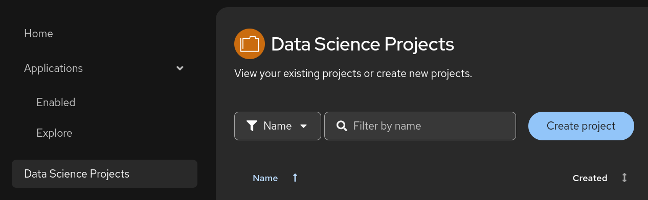Figure 1. Navigate to Data Science Projects in OpenShift AI Dashboard
Create a Data Science Project with the name quantization: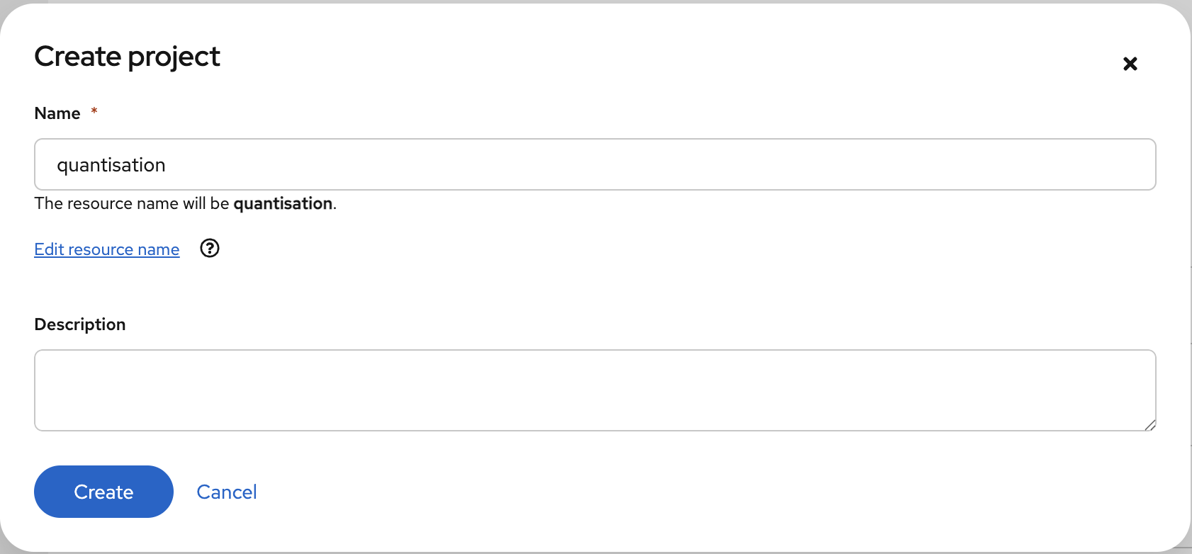

Figure 2. Create Data Science Project Named 'quantization'

Verify that your project appears in the Data Science Projects list with the name "quantization" and shows a "Ready" status.

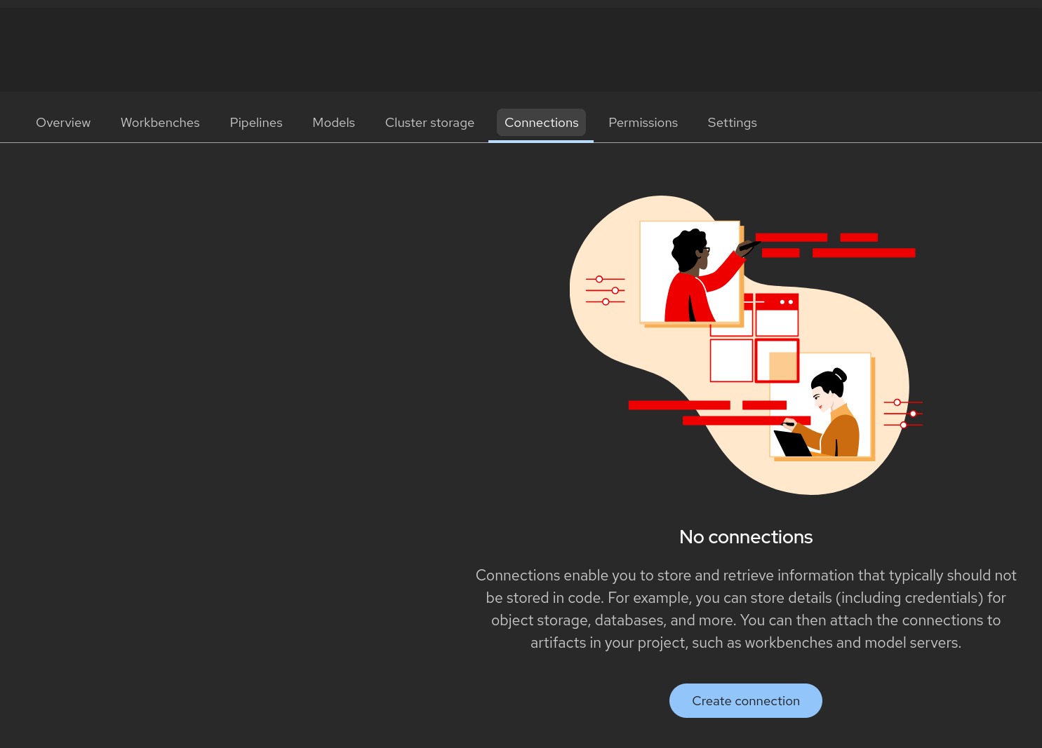
Creating a Data Connection for the Pipeline Server

Estimated time: 2-3 minutes

Now configure the data connection to link your pipeline server to MinIO storage.

Navigate to the quantization project in the OpenShift AI dashboard
Click Add Data Connection:

Figure 3. Add Data Connection Button in quantization Project

Select the connection type S3-compatible object storage -v1 and use the following values for configuring the MinIO connection:

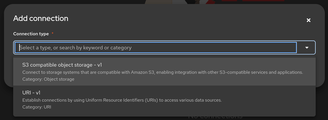Figure 4. Select S3-compatible Object Storage Connection Type
- Name:
  pipeline-connection
- Access Key:
  minio
- Secret Key:
  minio123
- Endpoint:
  http://minio.ic-shared-minio.svc.cluster.local:9000
- Region:
  none
- Bucket:
  pipelines
Verify your connection configuration matches this example:

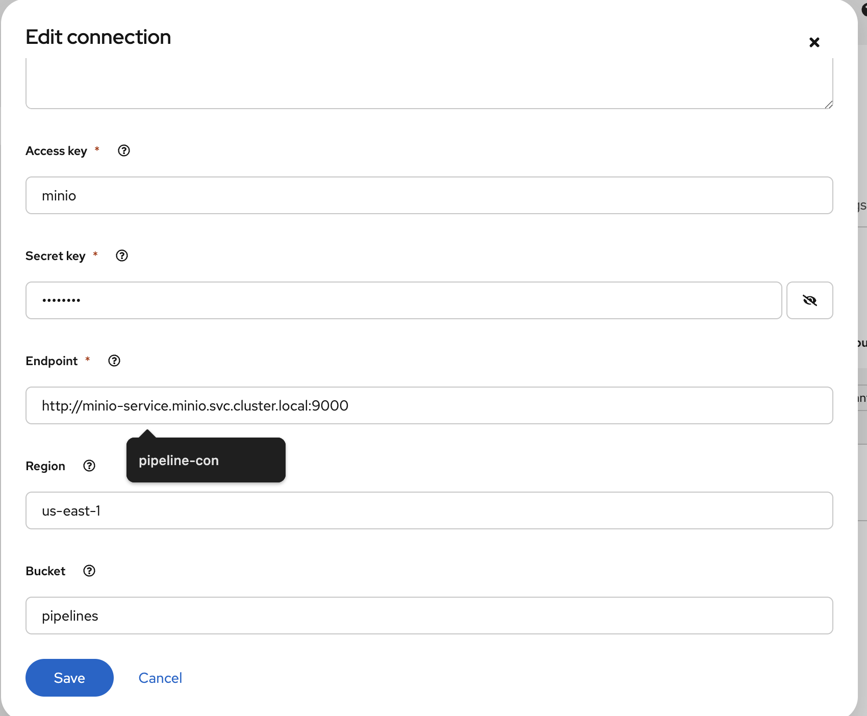Figure 5. Data Connection Configuration
Create a second Data Connection named minio-models:
- Use the same MinIO connection details as above
- Change the bucket name to models

Check that both data connections appear in your project:

pipeline-connection - connected to pipelines bucket
minio-models - connected to the bucket in which the model ibm-granite/granite-3.3-2b-instruct is available

Creating a Pipeline Server

Estimated time: 5-8 minutes

Create the pipeline server before setting up your workbench.

In the quantization project, navigate to Data science pipelines > Pipelines
Click Configure Pipeline Server:

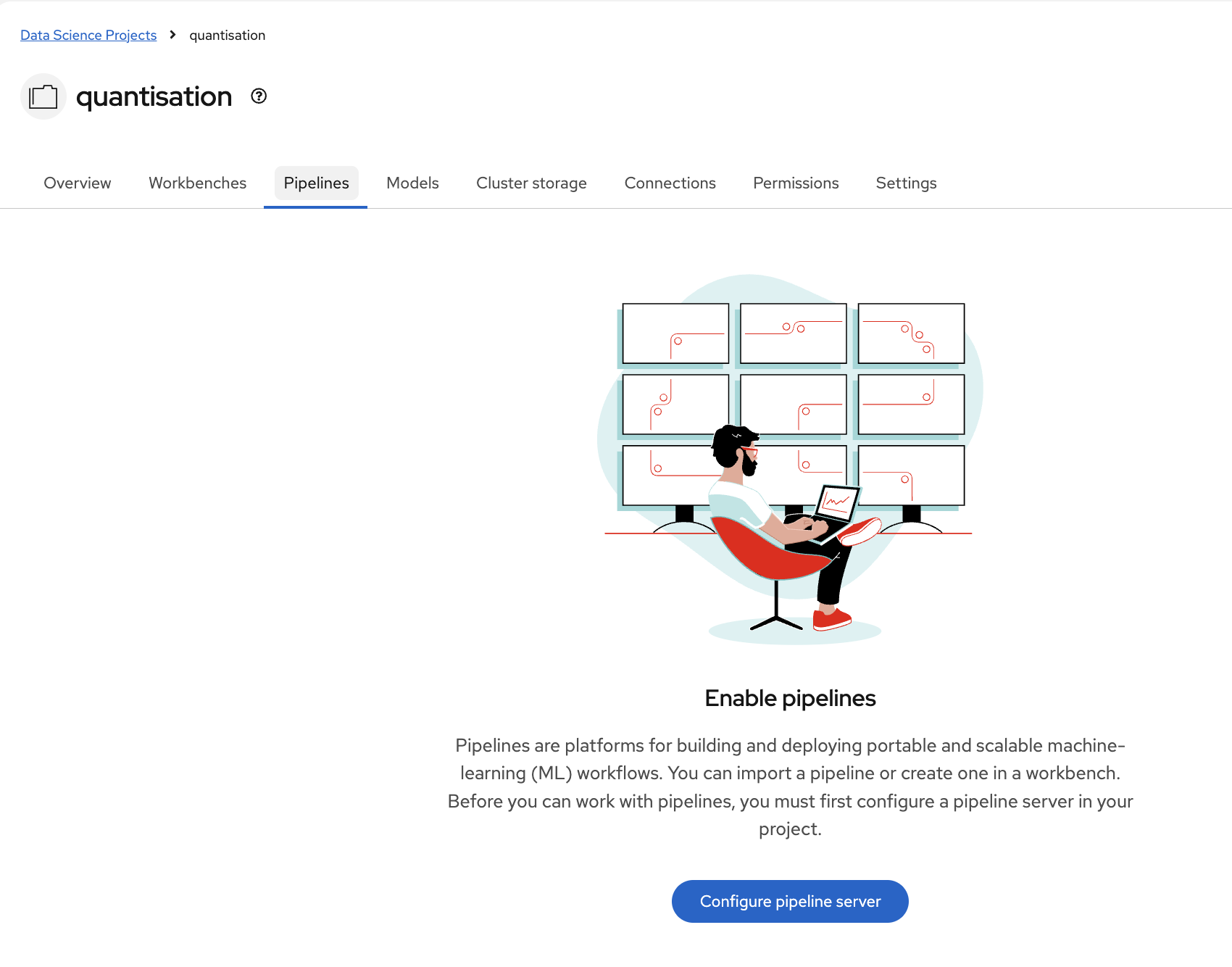Figure 6. Configure Pipeline Server Button Location
Select the pipeline-connection Data Connection you created earlier
Click Configure Pipeline Server:

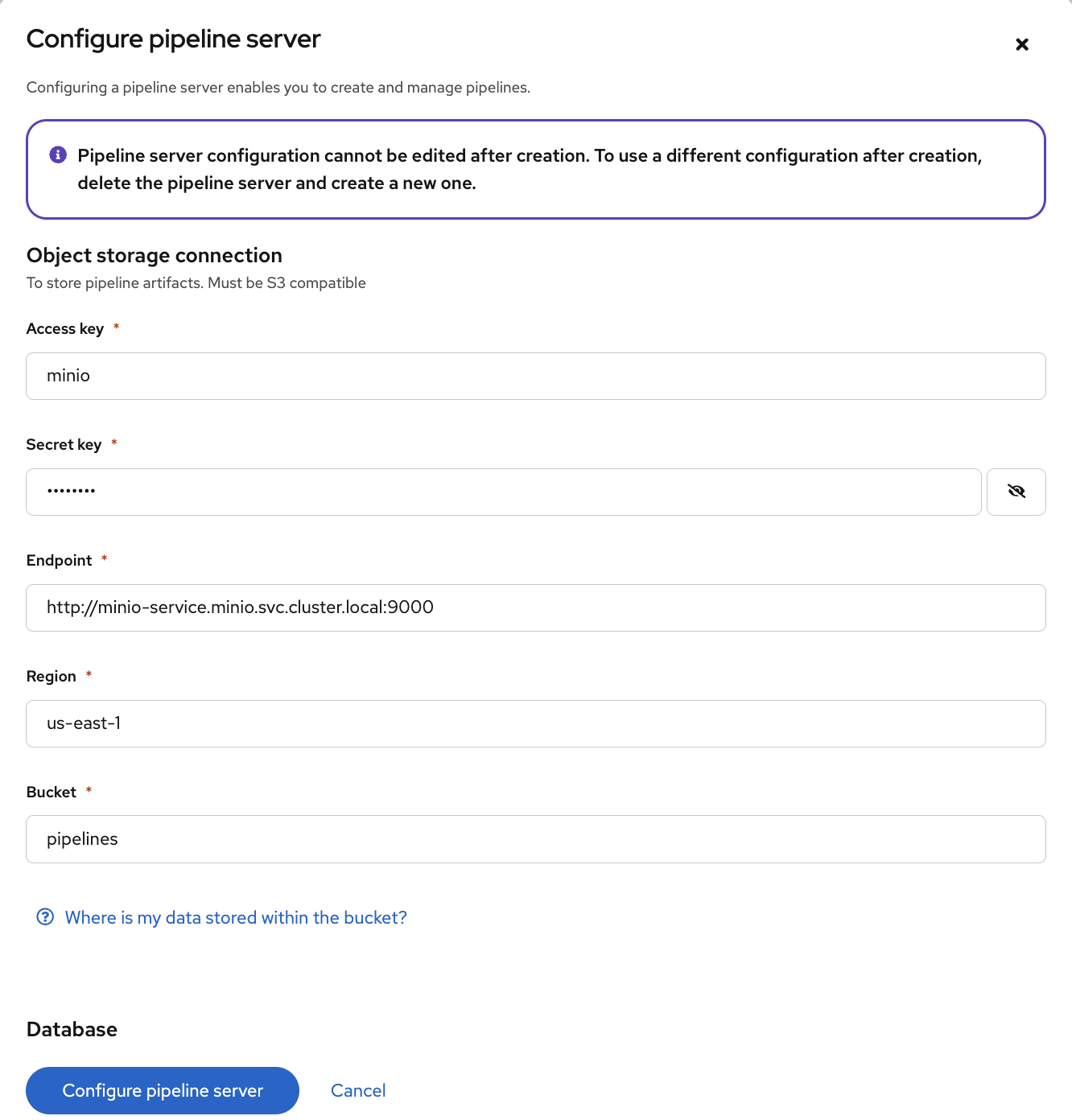Figure 7. Pipeline Server Configuration with Data Connection
Wait a few minutes for the pipeline server to deploy. The Pipelines section will display this status:

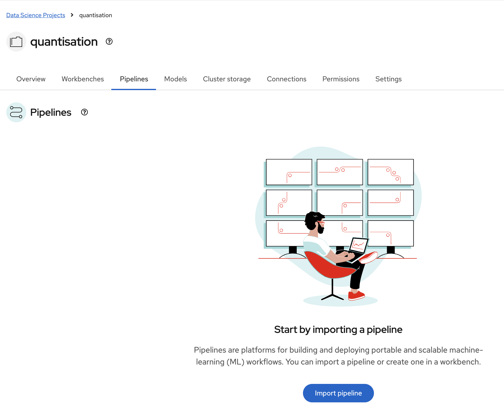Figure 8. Successfully Deployed Pipeline Server Status

This may take a few minutes to complete. There is no need to wait for the pipeline server to be ready. You may proceed to the next steps and check this later.

Verify that the pipeline server is running: * No error messages appear in the pipelines section

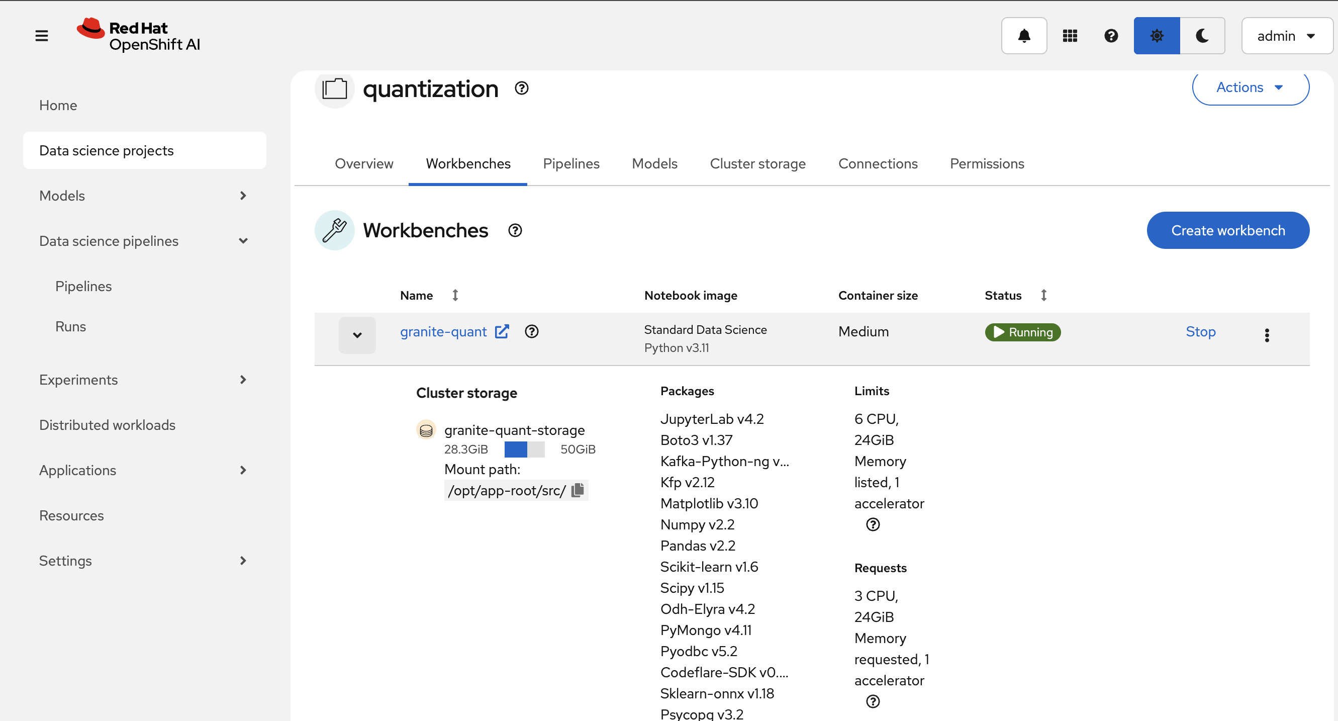
Creating a Workbench

Estimated time: 4-8 minutes (including startup)

With your Data Connection and Pipeline Server configured, you can now create the workbench environment.

In the quantization project, click Create a workbench: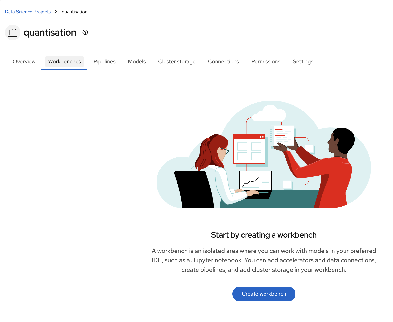

Figure 9. Create Workbench Button in quantization Project
Configure the workbench with these settings:
- Name: granite-quantization (or your preferred name)
- Image Selection: CUDA
- Container Size: Standard
- Accelerator: NVIDIA-GPU
- Number of accelerators: 2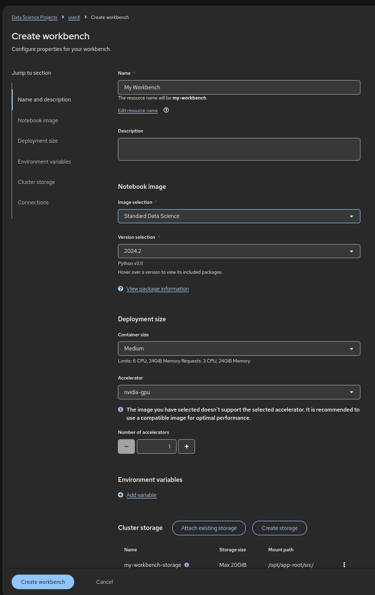
  
  Figure 10. Workbench Configuration Settings with GPU Accelerator
Attach the minio-models Data Connection:
- Click the Connections section
- Select Attach existing connections
- Click Attach for the minio-models connection
  
  Figure 11. Select Attach Existing Connections Option
  
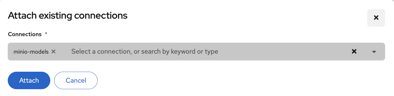  Figure 12. Attach minio-models Data Connection to Workbench
Click Create Workbench and wait for it to start
When the workbench status shows Running, click the link beside its name to open it:

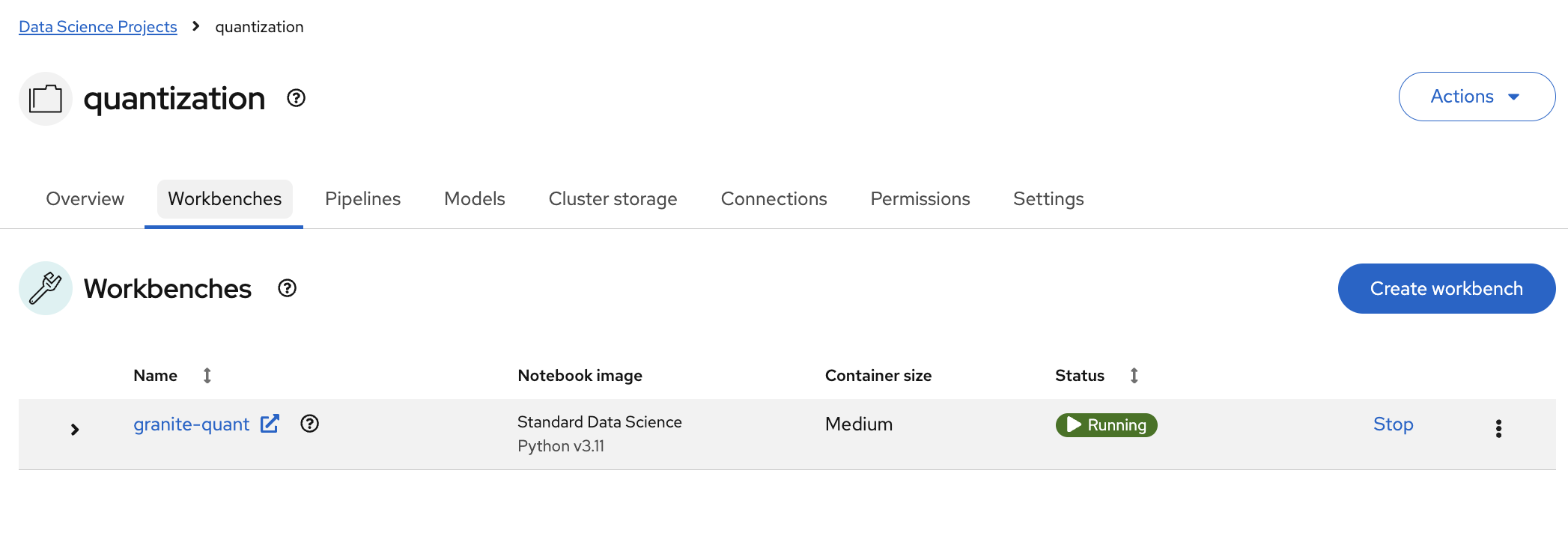Figure 13. Click Workbench Link to Launch Jupyter
Authenticate with your OpenShift login credentials
You will be asked to accept the following settings:

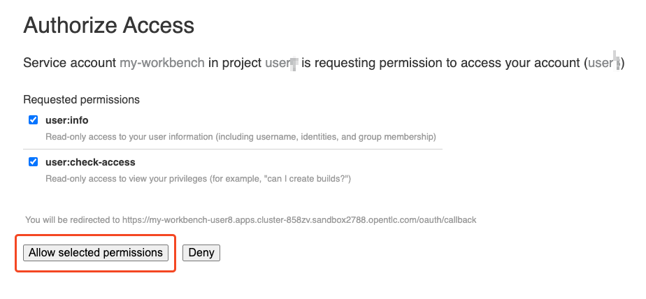Figure 14. Accept Jupyter Notebook Server Settings
After accepting the settings, the Jupyter interface will load:

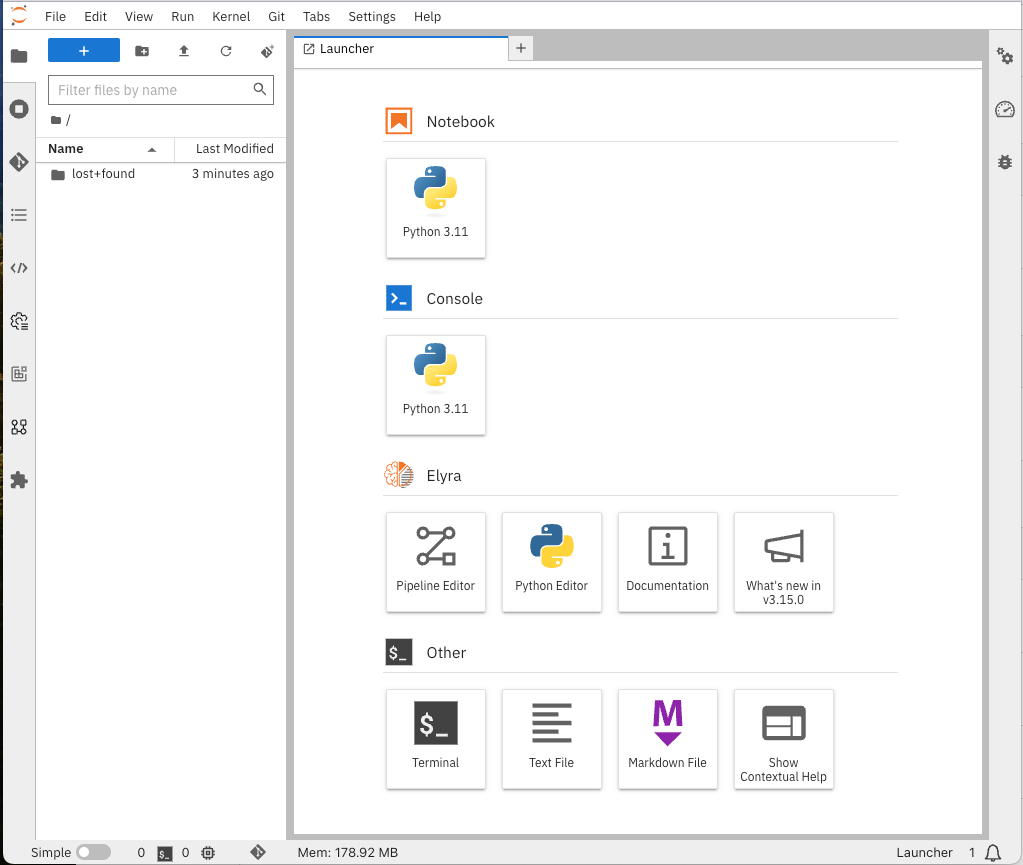Figure 15. Jupyter Interface Successfully Loaded

Confirm that:

Workbench status shows "Running"
Jupyter interface loads without errors
You can see the file browser and available kernels in the workbench
GPU is accessible (if applicable) from the workbench

Clone the repository

Estimated time: 1-2 minutes

With Jupyter running, clone the exercise repository to access the quantization notebooks.

Open the Git UI in Jupyter:

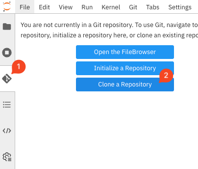Figure 16. Open Git Clone Interface in Jupyter
Specify the Git repository as:
```
https://github.com/redhat-ai-services/etx-llm-optimization-and-inference-leveraging.git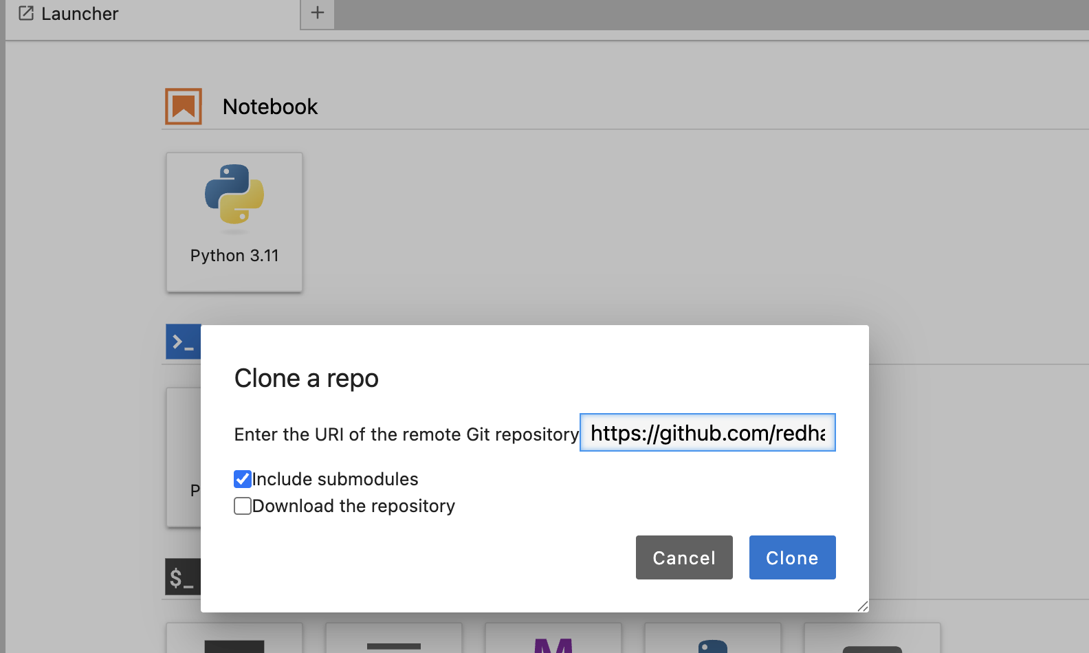
```
Figure 17. Successfully Cloned Repository in Jupyter Environment

You have now completed the setup and can proceed with the quantization exercise.

Before starting the quantization exercise, verify:

Repository is cloned successfully in Jupyter
/workshop_code/quantization/llm_compressor folder exists and contains:
- weight_activation_quantization.ipynb notebook
- minio.yaml file
- quantization_pipeline.py file
Data connections are accessible from the workbench environment
GPU resources are available for quantization tasks

Exercise: Quantize the Model with llm-compressor

Estimated time: 15-20 minutes (depending on model size and GPU performance)

Now you’ll perform the actual quantization using the provided Jupyter notebook.

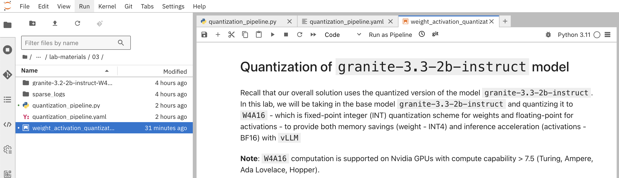
Navigate to the workshop_code/quantization/llm_compressor folder
Open the notebook weight_activation_quantization.ipynb:

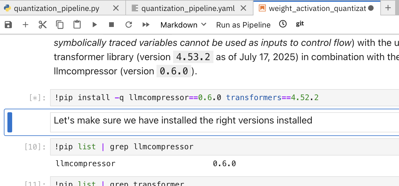
Figure 18. Weight Activation Quantization Notebook Ready to Execute

To execute the cells, you can select them and either click on the play icon or press Shift + Enter:

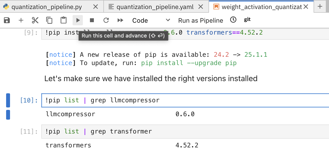
Figure 19. How to Execute Notebook Cells Using Play Button

When the cell is being executed, you can see [*]. Once the execution has completed, you will see a number instead of the *, e.g., [1]:

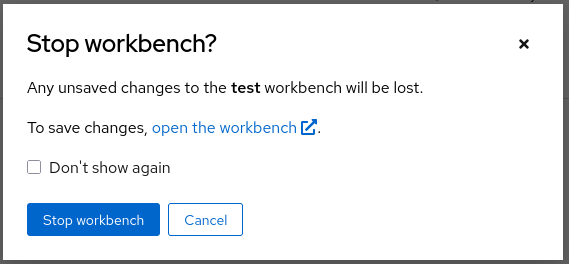
Figure 20. Cell Execution Status Indicators in Notebook

When you complete the notebook exercises, close the notebook and continue to the next module.

Once you complete this exercise and you no longer need the workbench, ensure you stop it so that the associated GPU gets freed and can be utilized to serve the model.

Figure 21. Access Workbench Actions Menu

Figure 22. Stop Workbench to Free GPU Resources