Model optimization
-
Deep dive presentation - vLLM and LLM Compressor
Challenges with running larger models
Even with the latest hardware like NVIDIA B200 GPUs offering up to 192GB of memory, the rapid increase in model sizes (e.g., GPT MoE 1.8T parameters) means that many state-of-the-art models cannot fit into a single GPU or even across multiple GPUs without optimization.
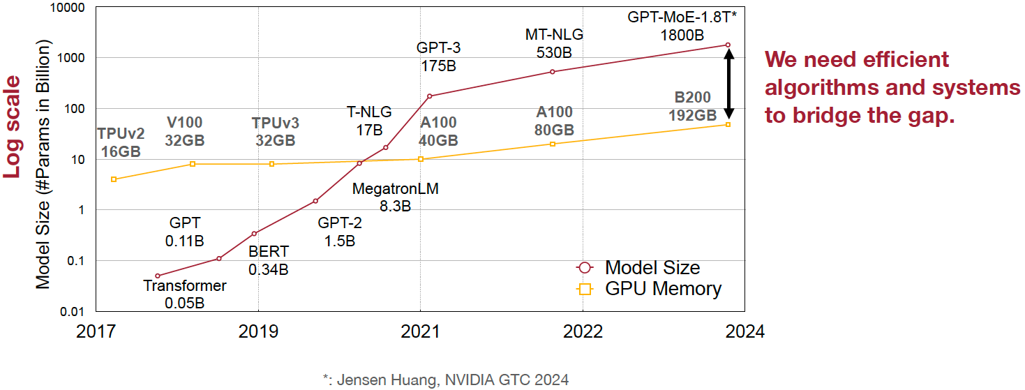
Give below are simple examples that shows how much memory is required just for storing parameters in GPUs for larger models.
Llama 4 Scout: 109B params
| Optimization | Params Size (GB) | GPUs Required |
|---|---|---|
BFloat16 |
109 * 2 ≈ 220GB |
3 x 80GB |
INT8/FP8 |
109 * 1 ≈ 109GB |
2 x 80GB |
INT4 |
109 * 0.5 ≈ 55GB |
1 x 80GB |
Llama 4 Maverick: 400B params
| Optimization | Params Size (GB) | GPUs Required |
|---|---|---|
BFloat16 |
400 * 2 ~= 800GB |
10 x 80GB ← requires multi-node! |
INT8/FP8 |
400 * 1 ~= 400GB |
5 x 80GB |
INT4 |
400 * 0.5 ~= 200GB |
3 x 80GB |
What optimized models offer:
-
Reduces GPU Memory requirements
-
Model parameters account for the majority of GPU RAM usage at typical sequence lengths.
-
Optimization allows you to allocate more memory to the KV cache, enabling longer context windows or larger batch sizes.
-
-
Accelerates linear layers
-
Minimizes data movement, which is a major bottleneck in large models.
-
Enables the use of low-precision tensor cores (as supported by the underlying hardwares), significantly speeding up matrix multiplications and inference.
-
-
Maintains model quality
-
Fine-grained quantization techniques can compress models with minimal or negligible impact on accuracy, preserving performance while reducing resource needs.
-
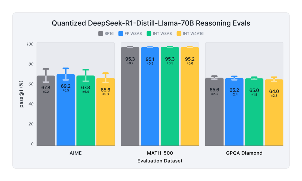
Below is an example of the DeepSeek R1 model, showing how different quantization methods impact evaluation results after compression. It’s important to note that not all quantization methods are equal and model quality can vary significantly depending on the quantization scheme used. So, it’s important to consider the impact on accuracy when choosing a quantization scheme.
In addition to the improvements described above, it also offers the following advantages:
-
Cost efficiency: Running large models requires expensive hardware. By optimizing and compressing models, you can reduce the required resources, leading to significant cost savings in both cloud and on-premise deployments.
-
Faster inference: Smaller, optimized models can process requests faster, reducing latency and improving user experience, especially in real-time applications.
-
Energy efficiency: Compressing models reduces the computational load, which in turn lowers power consumption and helps meet sustainability goals.
-
Deployment flexibility: Optimized models are easier to deploy on a wider range of devices, including edge devices and environments with limited resources.
-
Scalability: Smaller models allow you to serve more concurrent users or run more instances on the same hardware, improving scalability.
-
Bandwidth savings: Transferring large models over the network can be slow and costly. Compressed models are smaller and easier to distribute.
-
Regulatory and security constraints: Cases where data and models must remain on-premise or on specific hardware, optimization enables running advanced models within these constraints.
-
Enabling new use cases: By reducing the size and resource requirements, model optimization makes it feasible to use advanced LLMs in scenarios previously not possible, such as mobile, IoT, or embedded systems.
Quantization in practice
Quantization types in vLLM & LLM Compressor:
| Type of Quantization | What it does | Example impact | Quantization schemes supported |
|---|---|---|---|
Weight quantization |
Reduces the precision of model weights, lowering storage and memory requirements; LLM Compressor for weights quantization; Requires calibration dataset for weight quantization |
100B model: BFloat16 → 200GB, FP8 → 100GB |
W8A16, W4A16, WNA16 |
Weight and activation quantization |
Reduces model size and improves inference performance; LLM Compressor for weights quantization and vllm for activation quantization during inference; Requires calibration dataset for weight quantization |
Smaller activation memory footprint, faster inference |
W8A8, W4A8, W4A4 |
KV Cache quantization |
Reduced KV cache footprint & faster attention and crucial for large context workloads; Requires calibration dataset; LLM Compressor for scales calibration and vLLM to use the scales |
Enables longer context or larger batch sizes with same hardware |
FP8 |
Supported quantization schemes and when to use what?
| Format | Description | Use Case(s) | Recommended GPU type |
|---|---|---|---|
W4A16 |
4-bit weights, FP16 activations. High compression, fits small deployments; Requires calibration dataset for weight quantization. |
Memory-constrained inference at low QPS /online inferencing; edge devices; low memory/containerized apps. |
Recommended for any GPUs types. |
W8A8-INT8 |
8-bit weights, INT8 activations (per-token, runtime); Requires calibration dataset for weight quantization. |
High-QPS or offline serving; general purpose inference on any GPU; high-throughput inference on older GPUs. |
Recommended for NVIDIA GPUs with compute capability <8.9 (Ampere, Turing, Volta, Pascal, or older). |
W8A8-FP8 |
8-bit weights, FP8 activations (runtime). Preserves precision while gaining speed. Requires calibration dataset for weight quantization. |
High-QPS or offline serving; accuracy-sensitive with memory constraints; |
Recommended for NVIDIA GPUs with compute capability >=9.0 (Hopper and Blackwell). |
2:4 Sparsity (FP8 Weights/Activations) |
Structured sparsity + FP8 weights/activations. Uses sparsity acceleration. Very high performance. |
Speed-focused inference on modern hardware; |
Recommended for compute capability >=9.0 (Hopper and Blackwell). |
For a full list of supported hardware vs quantization scheme mapping, refer to the vLLM documentation.
Supported quantization methods/recipies and when to use what?
| Method | Description | Use case / Accuracy needs |
|---|---|---|
GPTQ |
Utilizes second-order layer-wise optimizations to prioritize important weights/activations and enables updates to remaining weights |
High accuracy recovery; best for scenarios where accuracy is critical and longer quantization time is acceptable |
AWQ |
Uses channelwise scaling to better preserve important outliers in weights and activations |
Moderate accuracy recovery; suitable when faster quantization is needed with reasonable accuracy |
SmoothQuant |
Smooths outliers in activations by folding them into weights, ensuring better accuracy for weight and activation quantized models |
Good accuracy recovery with minimal calibration time; can be combined with other methods for efficiency |
SparseGPT |
One‑shot pruning method that solves layer‑wise sparse regression to set weights to zero while readjusting survivors; supports unstructured sparsity up to ≈ 50–60 % without any retraining and 2 : 4 semi‑structured (N:M) sparsity for hardware‑friendly acceleration; can be stacked with low‑bit quantization |
When latency/throughput or memory footprint must drop quickly and some accuracy loss is acceptable: 2 : 4 mode on Hopper/Blackwell‑class GPUs for ~1.5–2× speed‑up with near‑AWQ accuracy on large‑scale models; small models (<7 B) may see noticeable drops |
Let’s help a client select the quantization method and scheme
| Question | Example client answer | How the client’s answer drives the decision |
|---|---|---|
1. Inference style Is the workload online (latency‑critical, interactive) or offline (throughput‑critical, batch)? |
e.g. “online customer‑service chatbot” |
• Online ⇒ Memory‑bandwidth bound ⇒ Weight‑only quantization (activations stay FP16). • Offline ⇒ Compute bound ⇒ Weight + activation quantization (both operands low‑precision). |
2. Target GPU architecture |
e.g. “Ampere A100” |
• Turing/Ampere have INT8 Tensor Cores ⇒ pick INT8 for speeds. • Hopper/H100 have native FP8 ⇒ pick FP8 (or INT8 if tooling is simpler). |
3. Expected concurrency / batch size Enough requests to saturate matrix‑mult units? |
e.g. “≈5 concurrent users; GPU often idle” |
• If GPU not fully busy, you gain more by cutting memory traffic (weight‑only). • If GPU fully busy, you gain more by lowering compute cost (weight + activation). |
4. Accuracy head‑room / SLA “How much accuracy can I lose?” |
e.g. “<0.5 pp drop allowed” |
Tight budgets push you toward higher‑accuracy methods (GPTQ, SmoothQuant + GPTQ). |
Example decision cheat sheet
| Chosen answers | Quantization scheme | Recommended method(s) | Why this combination? |
|---|---|---|---|
Online, Ampere/Turing, few users, strict latency |
W4 / W8 – A16 (weight-only) |
AWQ (fast), or GPTQ (max accuracy) |
Data-movement is the bottleneck; compute is "free". Weight-only avoids per-token FP16→INT8 converts on activations. |
Online, Hopper, few users |
W4 / W8 – A16 weight-only (still) |
AWQ or GPTQ |
Hopper can run FP8 activations, but if users are few, activation traffic is tiny—stick to weight-only. |
Offline, Ampere/Turing, large batch |
W8 – A8 (INT8/INT8) |
SmoothQuant + GPTQ (fold activation outliers, then weight-quant) |
Matrix-multiplication dominates; lowering both operands to INT8 doubles Tensor-Core throughput. |
Offline, Hopper, massive batch |
W8 – A8 or FP8/FP8 |
SmoothQuant + SparseGPT (optional pruning) |
Hopper’s FP8 Tensor Cores peak at ~2× A100 throughput. SmoothQuant tames activation outliers; SparseGPT can prune 2:4 (semi-structured) for more speed. |
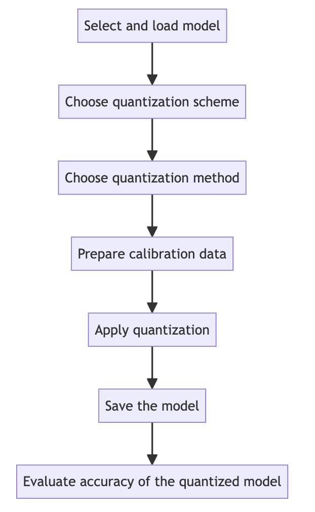
Quantization workflow
-
Model selection and loading
model = AutoModelForCausalLM.from_pretrained("your-model")
tokenizer = AutoTokenizer.from_pretrained("your-model")
-
Choosing the quantization scheme (Supported quantization schemes)
-
Choosing the quantization method (Supported quantization methods)
-
Preparing calibration data
-
Ensure the calibration data contains a high variety of samples to prevent overfitting towards a specific use case.
-
If the model was fine-tuned, use the sample datasets from the fine-tuning training data for calibration.
-
Employ the chat template or instruction template that the model was trained with.
-
Start with 512 samples for calibration data, and increase if accuracy drops.
-
Use a sequence length of 2048 as a starting point.
-
Tune key hyperparameters to the quantization algorithm:
-
dampening_fracsets how much influence the GPTQ algorithm has. Lower values can improve accuracy, but can lead to numerical instabilities that cause the algorithm to fail. -
actordersets the activation ordering. When compressing the weights of a layer, the order in which channels are quantized matters. Settingactorder="weight"can improve accuracy without added latency.
-
-
-
Applying quantization
-
Use oneshot API and provide the recipies to quantize and/or apply sparsity to the model given a dataset
-
from llmcompressor import oneshot

recipe = """
quant_stage:
    quant_modifiers:
        QuantizationModifier:
            ignore: ["lm_head"]
            config_groups:
                group_0:
                    weights:
                        num_bits: 8
                        type: float
                        strategy: tensor
                        dynamic: false
                        symmetric: true
                    input_activations:
                        num_bits: 8
                        type: float
                        strategy: tensor
                        dynamic: false
                        symmetric: true
                    targets: ["Linear"]
            kv_cache_scheme:
                num_bits: 8
                type: float
                strategy: tensor
                dynamic: false
                symmetric: true
"""

oneshot(
    model=model,
    dataset=ds,
    recipe=recipe,
    max_seq_length=MAX_SEQUENCE_LENGTH,
    num_calibration_samples=NUM_CALIBRATION_SAMPLES,
)
-
Saving the model
SAVE_DIR = MODEL_ID.split("/")[1] + "-FP8-KV"
model.save_pretrained(SAVE_DIR, save_compressed=True)
tokenizer.save_pretrained(SAVE_DIR)
-
Evaluating accuracy of the quantized model
lm_eval \
  --model vllm \
  --model_args pretrained=$MODEL,kv_cache_dtype=fp8,add_bos_token=True \
  --tasks gsm8k --num_fewshot 5 --batch_size auto